

The FOSDEM conference on February 3rd 2024 featured a presentation on Manticore Vector Search by Peter Zaitsev , co-founder of Manticore and Sergey Nikolaev , CEO of Manticore. This event showcased the latest about vector search in databases. For a closer look, a recording of Zaitsev's talk is available above. Below, you can see a more detailed summary of the topic in the form of an article.
Introduction
In the past two to three years, the database landscape has seen several key changes:
- A new category of 'vector databases' has emerged, featuring open-source platforms such as Milvus in 2019, Vespa in 2020, Weaviate in 2021, and Qdrant in 2022, as well as cloud solutions like Pinecone, introduced in 2019. These databases are dedicated to vector search, focusing on the use of various machine learning models. However, they may lack traditional database capabilities such as transactions, analytics, data replication, and so on
- Elasticsearch added vector search capabilities in 2019.
- Then from 2022 to 2023, established databases including Redis, OpenSearch, Cassandra, ClickHouse, Oracle, MongoDB, and Manticore Search, in addition to cloud services from Azure, Amazon AWS, and Cloudflare, started offering vector search functionality.
- Other well-known databases, like MariaDB, are in the process of integrating vector search capabilities*.
- For PostgreSQL users, there is the 'pgvector' extension which implements this functionality since 2021.
- While MySQL has not announced plans for native vector search functionality, proprietary extensions from providers such as PlanetScale and AlibabaCloud are available.

Vector space and vector similarity
Let’s discuss why so many databases recently enabled vector search functionality and what it is at all.
Let's begin with a tangible example. Consider two colors: red, with an RGB code of (255, 0, 0), and orange, with an RGB code of (255, 200, 152). To compare them, let’s plot them on a three-dimensional graph, where each point represents a different color, and the axes correspond to the red, green, and blue components of the colors. We then draw vectors from the origin of the graph to the points representing our colors. Now we have two vectors: one representing red and the other - orange.
If we want to find the similarity between these two colors, one approach could be to simply measure the angle between the vectors. This angle can vary from 0 to 90 degrees, or if we normalize it by taking the cosine, it will vary from 0 to 1. However, this method does not consider the magnitude of the vectors, which means that the cosine will yield the same value for colors A, A1, A2 even though they represent different shades.
To address this issue, we can use the cosine similarity formula, which accounts for vector lengths - the vectors dot product divided by the product of their magnitudes.

This concept is the essence of vector search. It's straightforward to visualize with colors, but now imagine that, instead of three color axes, we have a space with hundreds or thousands of dimensions, where each axis represents a specific feature of an object. While we can’t easily depict this on a slide or fully visualize it, mathematically it is feasible, and the principle remains the same: you have vectors in a multi-dimensional space and you compute the similarity between them.
There are a few other formulas to find vector similarity: for example the dot product similarity and the euclidean distance, but as the OpenAI API docs says, the difference between them typically doesn’t matter much.
Screenshot: https://platform.openai.com/docs/guides/embeddings/which-distance-function-should-i-use
Vector features: sparse vectors
So, an object may have various features. The color with Red, Green, and Blue components is the simplest example. In real life it’s typically more complex.
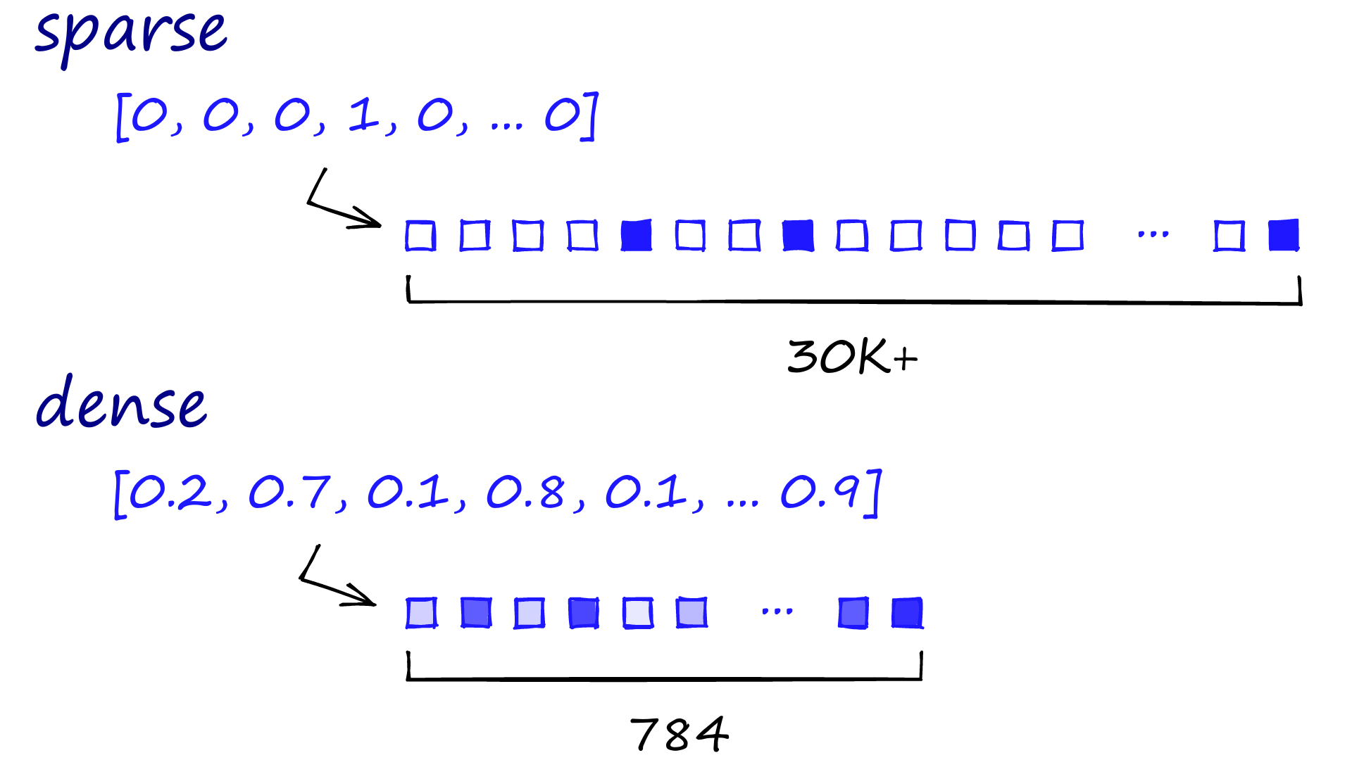
In text search, for instance, we may represent documents as high-dimensional vectors. This leads us to the concept of "Bag of Words." This model transforms text into vectors where each dimension corresponds to a unique word, and the value may be a binary indicator of the word’s presence, a count of occurrences, or a word weight based on its frequency and inversed document frequency (called TF-IDF), which reflects how important a word is to a document in a collection. This is so called sparse vector since most values are zero as most documents don’t have many words.
When talking about full-text search in libraries and search engines like Lucene , Elasticsearch , and Manticore Search , sparse vectors help make searches faster. Basically, you can make a special kind of index that ignores documents without the search term. So, you don't have to check every single document against your search each time. The sparse vectors are also easily understandable, they can be, in a sense, reverse-engineered. Each dimension corresponds to a specific clear feature, so we can trace back from our vector representation to the original text. This concept exists for already about 50 years.

Vector features: dense vectors
Traditional text search methods like TF-IDF , which have been around for decades, produce sparse word vectors that depend on term frequency. The main issue? They typically overlook the context in which words are used. For instance, the term “apple” could be associated with both fruit and the technology company without distinction, potentially ranking them similarly in a search.
But consider this analogy: In a vector space, which two objects would have a closer proximity: a cat and a dog, or a cat and a car? Traditional methods that generate sparse vectors — like the one shown at the top of the below image - may struggle to provide a meaningful answer. Sparse vectors are often high-dimensional, with most values being zero, representing the absence of most words in a given document or context.
Then came the revolution of deep learning, introducing contextual embeddings. These are dense vector representations, as illustrated by the lower part of the image. In contrast to sparse vectors, which may have tens of thousands of dimensions, dense vectors are lower-dimensional (such as 784 dimensions in the image) but packed with continuous values that capture nuanced semantic relationships. This means the same word can have different vector representations depending on its context, and different words can have similar vectors if they share contexts. Technologies like BERT and GPT use these dense vectors to capture complex language features including semantic relationships, distinguishing synonyms from antonyms, and comprehending irony and slang — tasks that were quite challenging for earlier methods.
Moreover, deep learning extends beyond text, enabling the processing of complex data like images, audio, and video. These can also be transformed into dense vector representations for tasks such as classification, recognition, and generation. The rise of deep learning coincided with the explosion in data availability and computational power, allowing the training of sophisticated models that uncover deeper and subtler patterns in data.

Embeddings
The vectors such models provide are called “embeddings”. It’s important to understand that unlike the sparse vectors shown previously, where each element can represent a clear feature like a word present in the document, each element of an embedding also represents a specific feature, but in most cases we don’t even know what the feature is.
For example, Jay Alammar made an interesting experiment
and used the GloVe model to vectorize Wikipedia and then visualized the values for some words with different colors. We can see here that:
- A consistent red line appears across various words, indicating similarity on one dimension, though the specific attribute it represents remains unidentified.
- Terms like "woman" and "girl" or "man" and "boy" display similarities across multiple dimensions, suggesting relatedness.
- Interestingly, "boy" and "girl" share similarities distinct from "woman" and "man," hinting at an underlying theme of youth.
- Except for one instance involving the term "water," all analyzed words pertain to people, with "water" serving to differentiate between conceptual categories.
- Distinct similarities between "king" and "queen" apart from other terms may suggest an abstract representation of royalty.

Image: https://jalammar.github.io/illustrated-word2vec/
So dense vector embeddings, generated through deep learning, capture a vast amount of information in a compact form. Unlike sparse vectors, every dimension of a dense embedding is generally non-zero and carries some semantic significance. This richness comes with a cost - with dense embeddings, since each dimension is densely populated with values, we can't simply skip documents that don't contain a specific term. Instead, we face the computational intensity of comparing the query vector with every document vector in the dataset. It's a brute-force approach that is naturally resource-intensive.
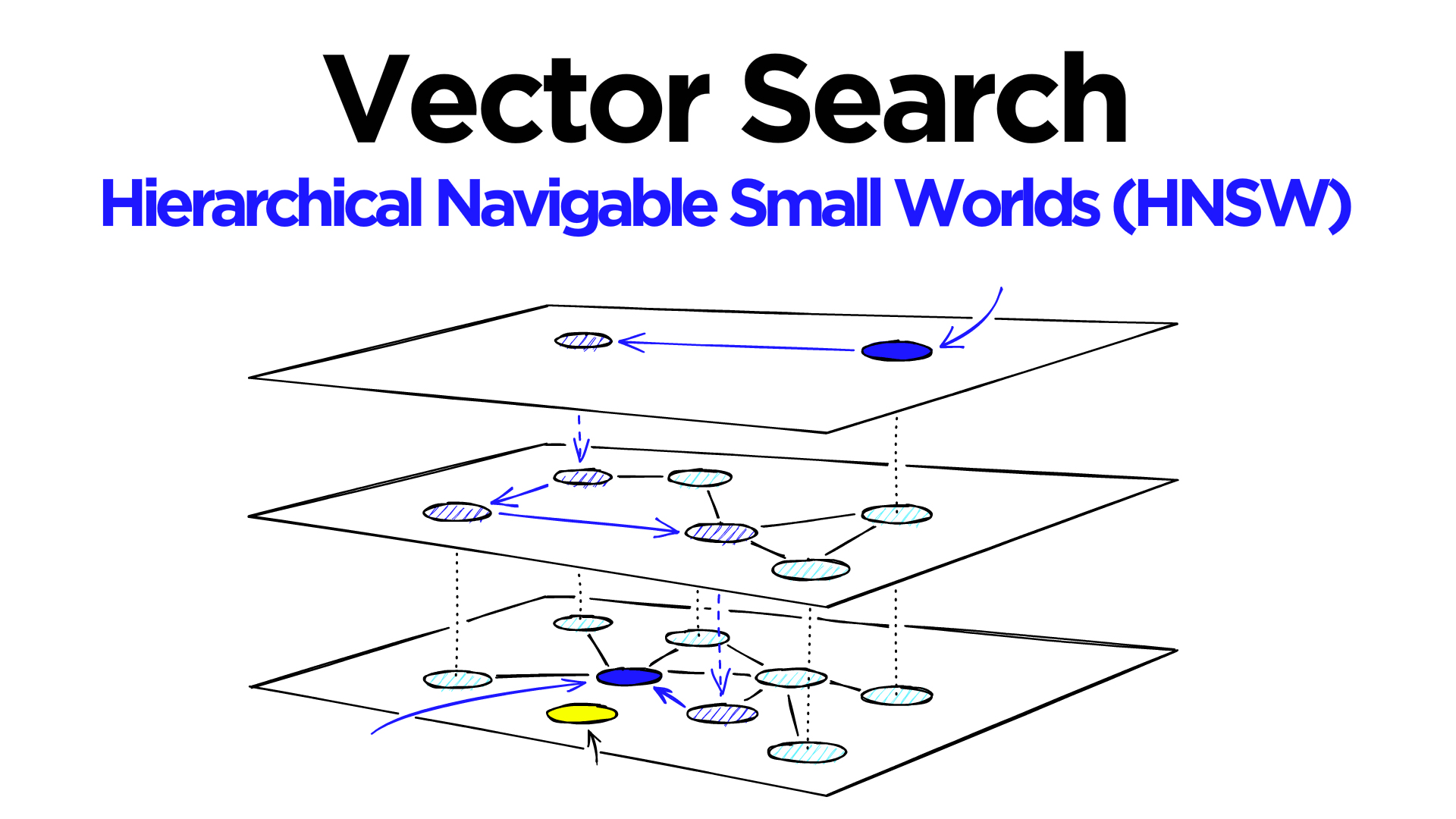
However, there have been developed specialized indexes tailored for dense vectors. These indexes, such as KD-trees, Ball trees, or more modern approaches like HNSW (Hierarchical Navigable Small World) graphs, are pretty smart, but they sometimes have to guess a bit to be fast. This guessing can mean they don't always get the answer 100% right. The most popular index that databases adopt is HNSW which stands for Hierarchical Navigable Small World. It’s used by the pgvector extension for Postgres, Lucene , Opensearch , Redis , SOLR , Cassandra , Manticore Search and Elasticsearch . Its algorithm builds a multi-layered graph structure. Each layer is a graph where each node (representing a data point) is connected to its closest neighbors. The bottom layer contains all nodes (data points), and each successive upper layer contains a subset of the nodes from the layer below. The topmost layer has the fewest nodes. Searching starts from the upper layers and gradually moves down to the lower layers. This hierarchical approach makes the search process efficient. In a nutshell HNSW like any other index just pregenerates some shortcuts that you then can use for faster query processing. There are other vector indexes, such as Annoy maintained by Spotify and others, each with its own set of pros and cons in terms of performance, resource consumption, and accuracy loss.

K-nearest neighbours
Vector search is actually an umbrella term that includes various tasks such as clustering and classification and others. But commonly, the first feature a database adds for vector search is the 'K-nearest neighbor search' (KNN), or its close relative, the 'Approximate nearest neighbor search' (ANN). It is appealing because it enables databases to find documents that are most similar to a given document’s vector which enhances databases with the powerful capabilities of a search engine, which they previously lacked.
Traditional search engines like Lucene, Elasticsearch, SOLR, and Manticore Search handle various natural language processing tasks — such as morphology, synonyms, stopwords, and exceptions — all aimed at finding documents that match a given query. KNN accomplishes a similar goal but through different means - just comparing the vectors associated with documents in the table that are usually provided by an external machine learning model.
Let's explore what a typical vector search looks like in databases, taking Manticore Search
as our example.
First, we create a table with a column titled image_vector:
create table test ( title text, image_vector float_vector knn_type='hnsw' knn_dims='4' hnsw_similarity='l2' );
This vector is of a float type
, which is important because databases that don’t support this data type must first add it, since dense vectors are usually stored in float arrays. At this time, you also usually configure the field by specifying the vector dimension size, vector index type, and its properties. For instance, we specify that we want to use the HNSW index, the vector will have a dimensionality of 5, and the similarity function will be l2, which is the Euclidean distance.
Then, we insert a few records into the table:
insert into test values ( 1, 'yellow bag', (0.653448,0.192478,0.017971,0.339821) ), ( 2, 'white bag', (-0.148894,0.748278,0.091892,-0.095406) );
Each record has a title and a corresponding vector, which, in a real-world scenario, could be the output from a deep learning model that encodes some form of high-dimensional data, such as an image or sound, an embedding from text, or something else from the OpenAI API. This operation stores the data in the database and may trigger rebuilding or adjusting the index.
Next, we perform a vector search by utilizing the KNN function :
select id, knn_dist() from test where knn ( image_vector, 5, (0.286569,-0.031816,0.066684,0.032926) );

+------+------------+
| id   | knn_dist() |
+------+------------+
|    1 | 0.28146550 |
|    2 | 0.81527930 |
+------+------------+
2 rows in set (0.00 sec)
Here we're querying the database to locate the vectors that are closest to our specified input vector. The numbers in parentheses define the particular vector we're seeking the nearest neighbors for. This step is critical for any database that aims to implement vector search capabilities. At this step the database can either utilize specific indexing methods, such as HNSW, or perform a brute-force search by comparing the query vector against each vector in the table to find the closest matches.
The results returned show the titles of the nearest vectors to our input vector and their respective distances from the query. Lower distance values indicate closer matches to the search query.

Embedding computation
Most databases and search engines so far rely on external embeddings. This means that when you insert a document, you must obtain its embedding from an external source beforehand and include it with the document's other fields. The same applies when searching for similar documents: if the search is for a user query rather than an existing document, you need to use a machine learning model to calculate an embedding for it, which is then passed to the database. This process can lead to compatibility issues, the need to manage additional data processing layers, and potential inefficiencies in search performance. The operational complexity of this approach is also higher than necessary. Along with the database, you may have to keep another service running to generate embeddings.
Some search engines like Opensearch, Elasticsearch, and Typesense are now making things easier by automatically creating embeddings. They can even use tools from other companies, like OpenAI, to do this. I think we'll see more of this soon. More databases will start to make embeddings on their own, which could really change how we search for and analyze data. This change means that databases will do more than just store data; they'll actually understand it. By using machine learning and AI, these databases will be smarter, able to predict and adapt, and handle data in more advanced ways.
Hybrid search approaches
Some search engines have adopted a method known as hybrid search, which combines traditional keyword-based search with advanced neural network techniques. Hybrid search models excel in situations that require both exact keyword matches, as provided by traditional search techniques, and broader context recognition, as offered by vector search capabilities. This balanced approach can enhance the accuracy of search results. For example, Vespa measured the accuracy of their hybrid search by comparing it to the classical BM25 ranking and the ColBERT model individually. In their approach, they used the classical BM25 as the first-phase ranking model and calculated the hybrid score only for the top-ranking K documents according to the BM25 model. It was found that the hybrid search mode outperformed each of them in most tests.
Another simpler method is Reciprocal Rank Fusion (RRF), a technique that combines rankings from different search algorithms. RRF calculates a score for each item based on its rank in each list, where higher rankings receive better scores. The score is determined by the formula 1 / (rank + k), where 'rank' is the item's position in the list, and 'k' is a constant used to adjust the influence of lower rankings. By summing these modified reciprocal ranks from each source, RRF emphasizes consensus among different systems. This method blends the strengths of various algorithms, leading to more robust and comprehensive search results.

Table: https://blog.vespa.ai/improving-zero-shot-ranking-with-vespa-part-two/
Formula: https://plg.uwaterloo.ca/~gvcormac/cormacksigir09-rrf.pdf
Conclusion
Vector search is more than just a concept or a niche functionality of search engines; it's a practical tool transforming how we retrieve data. In recent years, the database field has seen major changes, with the rise of new vector-focused databases and established ones adding vector search features. This reflects a strong need for more advanced search functions, a need that vector search can meet. Advanced indexing methods, like HNSW, have made vector search faster.
Looking ahead, we expect databases to do more than just support vector search; they'll likely create embeddings themselves. This will make databases simpler to use and more powerful, turning them from basic storage spaces into smart systems that can understand and analyze data. In short, vector search is a significant shift in data management and retrieval, marking an exciting development in the field.